Introduction
Software
Applications
Detectors
GM-10
GM-45
GM-90
Accessories
Test Source
Battery Box
Coincidence Box
Anti-Coincidence
GMI Interface
Air Sampler
Download
Linux
Users Group
Interfacing
Raspberry Pi
Random Numbers
Safety Uses
Radiation Info
Specifications
FAQ
Articles
Experiments
Rad Map
Links
Secure Order
Detectors
Contact
Radiation Counting Statistics With The GM-10
The decay of radioactive atoms is a random event. This means that, if we know the activity (decays per second) of a source of radiation, we only know the average decay rate. We cannot specify the exact decay rate, nor when a particular atom will decay. We can only compute probabilities.The number of decays per unit of time of a radioactive source is a Poisson Distribution. For example, if a source has an activity of 100 Bequerels (decays per second), the source will not always produce exactly 100 decays per second, but an average of 100 decays per second. The standard deviation is equal to the square root of the number of decays. In this case the square root of 100 is 10, so the standard deviation is 10.
The standard deviation allows us to determine with what confidence we can predict the actual number of decays per second (or other time period) will be. The following table shows the confidence for varying standard deviations:
1 sigma	0.6826895
2 sigma	0.9544997
3 sigma	0.9973002
4 sigma	0.9999366
5 sigma	0.9999994
What does this mean? In our case above, the standard deviation (1 sigma) was 10 counts, with an average counting rate of 100 counts per second. That means that 68% of the time, we would expect the number of counts measured to lie withing 100 +/-10 or from 90 to 110. We would expect to be within a range of 100 +/-20 counts 95% of the time, etc.
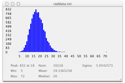
It's quite easy to do an experiment with the GM-10 to test this out. You need a source of radiation, our vaseline glass beads work quite well, and give a nominal reading of about 200 CPM. At that rate, we would expect a standard devaition of about 14.
Set the Rad software to record the reading each minute. The resulting data file can be analyzed. Our Histogram software (included with the Rad package) will compute the average and standard deviation values, as well as sort the readings into bins, and display the resulting histogram. Data should be collected for as long as possible, to get results closest to theory. It's all counting statistics, after all!
Here are the results of an experiment we did:

If you'd like to see our actual data, here is the raw data and here is the binned data. The histogram software that comes with the GM-10 and GM-45 detectors automatically bins recorded data and produces such a graph.